梯度提升树算法流程（梯度提升算法的理解）



梯度下降是一种优化算法，遵循目标函数的负梯度以定位函数的最小值。

梯度下降的局限性是，所有输入变量都使用单个步长（学习率）。像AdaGrad和RMSProp这样的梯度下降的扩展会更新算法，以对每个输入变量使用单独的步长，但可能会导致步长迅速减小到非常小的值。自适应运动估计算法（Adam）是梯度下降的扩展，是AdaGrad和RMSProp等技术的自然继承者，该技术可自动为目标函数的每个输入变量调整学习率，并通过使用以指数方式降低梯度的移动平均值以更新变量。

在本教程中，您将发现如何从头开始使用Adam优化算法开发梯度下降。完成本教程后，您将知道：

• 梯度下降是一种优化算法，它使用目标函数的梯度来导航搜索空间。
• 可以通过使用称为Adam的偏导数的递减平均值，将梯度下降更新为对每个输入变量使用自动自适应步长。
• 如何从头开始实施Adam优化算法并将其应用于目标函数并评估结果。

教程概述

本教程分为三个部分：他们是：

• 梯度下降
• Adam优化算法
• Adam梯度下降
  二维测试问题
  Adam的梯度下降优化
  Adam可视化

梯度下降

梯度下降是一种优化算法。它在技术上称为一阶优化算法，因为它明确利用了目标目标函数的一阶导数。一阶导数，或简称为“导数”，是目标函数在特定点（例如，点）上的变化率或斜率。用于特定输入。如果目标函数采用多个输入变量，则将其称为多元函数，并且可以将输入变量视为向量。反过来，多元目标函数的导数也可以视为向量，通常称为梯度。

梯度：多元目标函数的一阶导数。

对于特定输入，导数或梯度指向目标函数最陡峭的上升方向。

梯度下降是指一种最小化优化算法，该算法遵循目标函数的下坡梯度负值来定位函数的最小值。梯度下降算法需要一个正在优化的目标函数和该目标函数的导数函数。目标函数f（）返回给定输入集合的分数，导数函数f'（）给出给定输入集合的目标函数的导数。梯度下降算法需要问题中的起点（x），例如输入空间中的随机选择点。

假设我们正在最小化目标函数，然后计算导数并在输入空间中采取一步，这将导致目标函数下坡运动。下坡运动是通过首先计算输入空间中的运动量来进行的，计算方法是将步长（称为alpha或学习率）乘以坡度。然后从当前点减去该值，以确保我们逆梯度移动或向下移动目标函数。

x（t）= x（t-1）–step* f'（x（t-1））

在给定点的目标函数越陡峭，梯度的幅度越大，反过来，在搜索空间中采取的步伐也越大。使用步长超参数来缩放步长的大小。

步长（alpha）：超参数，控制算法每次迭代时相对于梯度在搜索空间中移动多远。

如果步长太小，则搜索空间中的移动将很小，并且搜索将花费很长时间。如果步长太大，则搜索可能会在搜索空间附近反弹并跳过最优值。

现在我们已经熟悉了梯度下降优化算法，下面让我们看一下Adam算法。

Adam优化算法

自适应运动估计算法（简称“Adam”）是梯度下降优化算法的扩展。Diederik Kingma和Jimmy Lei Ba在2014年发表的题为“Adam：随机优化方法”的论文中描述了该算法。Adam旨在加速优化过程，例如减少达到最佳状态所需的功能评估次数，或提高优化算法的功能，例如产生更好的最终结果。这是通过为每个要优化的输入参数计算步长来实现的。重要的是，每个步长都将根据每个变量遇到的梯度（偏导数）自动调整搜索过程的吞吐量。

让我们逐步介绍该算法的每个元素。首先，对于作为搜索一部分而被优化的每个参数，我们必须维持一个矩矢量和指数加权无穷大范数，分别称为m和v（真是希腊字母nu）。在搜索开始时将它们初始化为0.0。

m = 0

v = 0

该算法在从 t=1 开始的时间t内迭代执行，并且每次迭代都涉及计算一组新的参数值x，例如。从 x（t-1） 到 x（t） 。如果我们专注于更新一个参数，这可能很容易理解该算法，该算法概括为通过矢量运算来更新所有参数。首先，计算当前时间步长的梯度（偏导数）。

g（t）= f'（x（t-1））

接下来，使用梯度和超参数 beta1 更新第一时刻。

m（t）= beta1 * m（t-1）+（1 – beta1）* g（t）

然后，使用平方梯度和超参数 beta2 更新第二时刻。

v（t）= beta2 * v（t-1）+（1 – beta2）* g（t）^ 2

由于第一和第二力矩是用零值初始化的，所以它们是有偏的。接下来，对第一力矩和第二力矩进行偏差校正，并以第一力矩为起点：

mhat（t）= m（t）/（1 – beta1（t））

然后第二个时刻：

vhat（t）= v（t）/（1 – beta2（t））

注意， beta1（t） 和 beta2（t） 指的是 beta1 和 beta2 超参数，它们在算法的迭代过程中按时间表衰减。可以使用静态衰减时间表，尽管该论文建议以下内容：

beta1（t）= beta1 ^ t

beta2（t）= beta2 ^ t

最后，我们可以为该迭代计算参数的值。

x（t）= x（t-1）– alpha * mhat（t）/（sqrt（vhat（t））+ eps）

其中 alpha 是步长超参数， eps 是一个较小的值（ epsilon ），例如 1e-8 ，可确保我们不会遇到被零除的误差，而 sqrt（） 是平方根函数。

注意，可以使用对本文中列出的更新规则进行更有效的重新排序：

alpha（t）= alpha * sqrt（1 – beta2（t））/（1 – beta1（t）） x（t）= x（t-1）– alpha（t）* m（t）/（sqrt（v（t））+ eps）

回顾一下，该算法有三个超参数，它们是：

• alpha：初始步长（学习率），典型值为0.001。
• beta1：第一个动量的衰减因子，典型值为0.9。
• beta2：无穷大范数的衰减因子，典型值为0.999。

接下来，让我们看看如何在Python中从头开始实现该算法。

Adam梯度下降

在本节中，我们将探讨如何使用Adam实现梯度下降优化算法。

二维测试问题

首先，让我们定义一个优化函数。我们将使用一个简单的二维函数，该函数将每个维的输入平方，并定义有效输入的范围（从-1.0到1.0）。

下面的 Objective（） 函数实现了此功能

# objective function
def objective(x, y):
 return x2.0 + y2.0

我们可以创建数据集的三维图，以了解响应面的曲率。下面列出了绘制目标函数的完整示例。

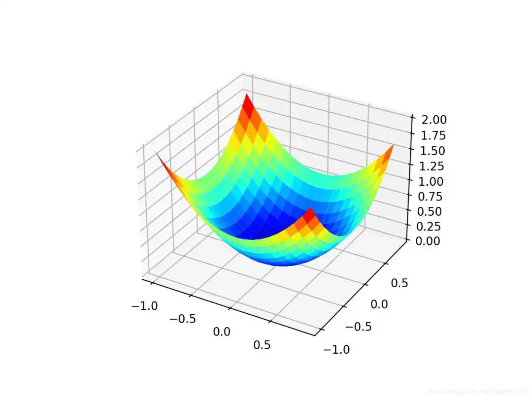
# 3d plot of the test function
from numpy import arange
from numpy import meshgrid
from matplotlib import pyplot
 
# objective function
def objective(x, y):
 return x2.0 + y2.0
 
# define range for input
r_min, r_max = -1.0, 1.0
# sample input range uniformly at 0.1 increments
xaxis = arange(r_min, r_max, 0.1)
yaxis = arange(r_min, r_max, 0.1)
# create a mesh from the axis
x, y = meshgrid(xaxis, yaxis)
# compute targets
results = objective(x, y)
# create a surface plot with the jet color scheme
figure = pyplot.figure()
axis = figure.gca(projection='3d')
axis.plot_surface(x, y, results, cmap='jet')
# show the plot
pyplot.show()

运行示例将创建目标函数的三维表面图。我们可以看到全局最小值为 f（0，0）= 0 的熟悉的碗形状。

我们还可以创建函数的二维图。这在以后要绘制搜索进度时会很有帮助。下面的示例创建目标函数的轮廓图。

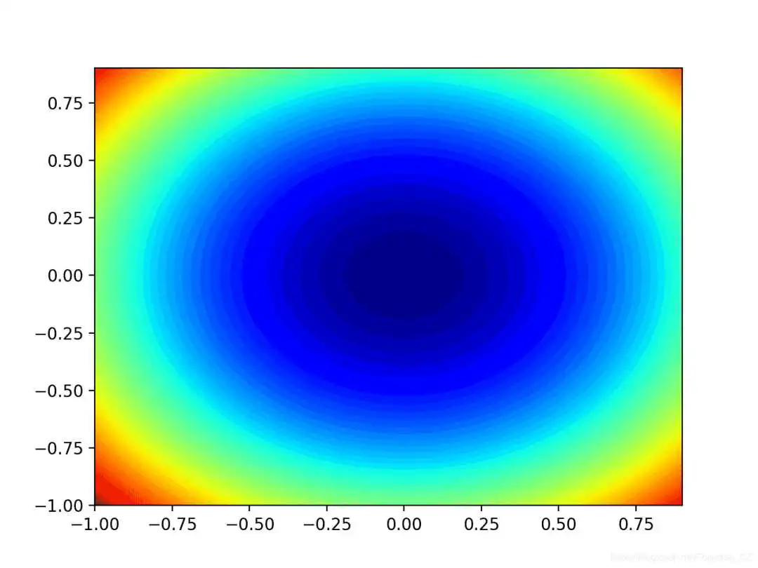
# contour plot of the test function
from numpy import asarray
from numpy import arange
from numpy import meshgrid
from matplotlib import pyplot
 
# objective function
def objective(x, y):
 return x2.0 + y2.0
 
# define range for input
bounds = asarray([[-1.0, 1.0], [-1.0, 1.0]])
# sample input range uniformly at 0.1 increments
xaxis = arange(bounds[0,0], bounds[0,1], 0.1)
yaxis = arange(bounds[1,0], bounds[1,1], 0.1)
# create a mesh from the axis
x, y = meshgrid(xaxis, yaxis)
# compute targets
results = objective(x, y)
# create a filled contour plot with 50 levels and jet color scheme
pyplot.contourf(x, y, results, levels=50, cmap='jet')
# show the plot
pyplot.show()

运行示例将创建目标函数的二维轮廓图。我们可以看到碗的形状被压缩为以颜色渐变显示的轮廓。我们将使用该图来绘制在搜索过程中探索的特定点。

现在我们有了一个测试目标函数，让我们看一下如何实现Adam优化算法。

Adam梯度下降优化

我们可以将带有Adam的梯度下降应用于测试问题。首先，我们需要一个函数来计算此函数的导数。

f（x）= x ^ 2

f'（x）= x * 2

x ^ 2 的导数在每个维度上均为 x * 2 。 derived（） 函数在下面实现了这一点。

# derivative of objective function
def derivative(x, y):
 return asarray([x * 2.0, y * 2.0])

接下来，我们可以实现梯度下降优化。首先，我们可以选择问题范围内的随机点作为搜索的起点。假定我们有一个数组，该数组定义搜索范围，每个维度一行，并且第一列定义最小值，第二列定义维度的最大值。

# generate an initial point
x = bounds[:, 0] + rand(len(bounds)) * (bounds[:, 1] - bounds[:, 0])
score = objective(x[0], x[1])

接下来，我们需要将第一时刻和第二时刻初始化为零。

# initialize first and second moments
m = [0.0 for _ in range(bounds.shape[0])]
v = [0.0 for _ in range(bounds.shape[0])]

然后，我们运行由“ n_iter”超参数定义的算法的固定迭代次数。

...
# run iterations of gradient descent
for t in range(n_iter):
 ...

第一步是使用导数（）函数计算当前解决方案的梯度。

# calculate gradient
gradient = derivative(solution[0], solution[1])

第一步是计算当前参数集的导数。

# calculate gradient g(t)
g = derivative(x[0], x[1])

接下来，我们需要执行Adam更新计算。为了提高可读性，我们将使用命令式编程样式一次执行一个变量的这些计算。

在实践中，我建议使用NumPy向量运算以提高效率。

...
# build a solution one variable at a time
for i in range(x.shape[0]):
 ...

首先，我们需要计算力矩。

# m(t) = beta1 * m(t-1) + (1 - beta1) * g(t)
m[i] = beta1 * m[i] + (1.0 - beta1) * g[i]

然后是第二个时刻。

# v(t) = beta2 * v(t-1) + (1 - beta2) * g(t)^2
v[i] = beta2 * v[i] + (1.0 - beta2) * g[i]2

然后对第一和第二时刻进行偏差校正。

# mhat(t) = m(t) / (1 - beta1(t))
mhat = m[i] / (1.0 - beta1(t+1))
# vhat(t) = v(t) / (1 - beta2(t))
vhat = v[i] / (1.0 - beta2(t+1))

然后最后是更新的变量值。

# x(t) = x(t-1) - alpha * mhat(t) / (sqrt(vhat(t)) + eps)
x[i] = x[i] - alpha * mhat / (sqrt(vhat) + eps)

然后，针对要优化的每个参数重复此操作。在迭代结束时，我们可以评估新的参数值并报告搜索的性能。

# evaluate candidate point
score = objective(x[0], x[1])
# report progress
print('>%d f(%s) = %.5f' % (t, x, score))

我们可以将所有这些结合到一个名为 adam（） 的函数中，该函数采用目标函数和派生函数的名称以及算法超参数，并返回在搜索及其评估结束时找到的最佳解决方案。

下面列出了完整的功能。

# gradient descent algorithm with adam
def adam(objective, derivative, bounds, n_iter, alpha, beta1, beta2, eps=1e-8):
 # generate an initial point
 x = bounds[:, 0] + rand(len(bounds)) * (bounds[:, 1] - bounds[:, 0])
 score = objective(x[0], x[1])
 # initialize first and second moments
 m = [0.0 for _ in range(bounds.shape[0])]
 v = [0.0 for _ in range(bounds.shape[0])]
 # run the gradient descent updates
 for t in range(n_iter):
  # calculate gradient g(t)
  g = derivative(x[0], x[1])
  # build a solution one variable at a time
  for i in range(x.shape[0]):
   # m(t) = beta1 * m(t-1) + (1 - beta1) * g(t)
   m[i] = beta1 * m[i] + (1.0 - beta1) * g[i]
   # v(t) = beta2 * v(t-1) + (1 - beta2) * g(t)^2
   v[i] = beta2 * v[i] + (1.0 - beta2) * g[i]2
   # mhat(t) = m(t) / (1 - beta1(t))
   mhat = m[i] / (1.0 - beta1(t+1))
   # vhat(t) = v(t) / (1 - beta2(t))
   vhat = v[i] / (1.0 - beta2(t+1))
   # x(t) = x(t-1) - alpha * mhat(t) / (sqrt(vhat(t)) + eps)
   x[i] = x[i] - alpha * mhat / (sqrt(vhat) + eps)
  # evaluate candidate point
  score = objective(x[0], x[1])
  # report progress
  print('>%d f(%s) = %.5f' % (t, x, score))
 return [x, score]

注意：为了提高可读性，我们有意使用列表和命令式编码样式，而不是矢量化操作。随意将实现改编为带有NumPy数组的矢量化实现，以实现更好的性能。

然后，我们可以定义我们的超参数并调用 adam（） 函数来优化我们的测试目标函数。

在这种情况下，我们将使用算法的60次迭代，初始步长为0.02， beta1 和 beta2 值分别为0.8和0.999。经过一些反复试验后，发现了这些超参数值。

# seed the pseudo random number generator
seed(1)
# define range for input
bounds = asarray([[-1.0, 1.0], [-1.0, 1.0]])
# define the total iterations
n_iter = 60
# steps size
alpha = 0.02
# factor for average gradient
beta1 = 0.8
# factor for average squared gradient
beta2 = 0.999
# perform the gradient descent search with adam
best, score = adam(objective, derivative, bounds, n_iter, alpha, beta1, beta2)
print('Done!')
print('f(%s) = %f' % (best, score))

综合所有这些，下面列出了使用 Adam 进行梯度下降优化的完整示例。

# gradient descent optimization with adam for a two-dimensional test function
from math import sqrt
from numpy import asarray
from numpy.random import rand
from numpy.random import seed
 
# objective function
def objective(x, y):
 return x2.0 + y2.0
 
# derivative of objective function
def derivative(x, y):
 return asarray([x * 2.0, y * 2.0])
 
# gradient descent algorithm with adam
def adam(objective, derivative, bounds, n_iter, alpha, beta1, beta2, eps=1e-8):
 # generate an initial point
 x = bounds[:, 0] + rand(len(bounds)) * (bounds[:, 1] - bounds[:, 0])
 score = objective(x[0], x[1])
 # initialize first and second moments
 m = [0.0 for _ in range(bounds.shape[0])]
 v = [0.0 for _ in range(bounds.shape[0])]
 # run the gradient descent updates
 for t in range(n_iter):
  # calculate gradient g(t)
  g = derivative(x[0], x[1])
  # build a solution one variable at a time
  for i in range(x.shape[0]):
   # m(t) = beta1 * m(t-1) + (1 - beta1) * g(t)
   m[i] = beta1 * m[i] + (1.0 - beta1) * g[i]
   # v(t) = beta2 * v(t-1) + (1 - beta2) * g(t)^2
   v[i] = beta2 * v[i] + (1.0 - beta2) * g[i]2
   # mhat(t) = m(t) / (1 - beta1(t))
   mhat = m[i] / (1.0 - beta1(t+1))
   # vhat(t) = v(t) / (1 - beta2(t))
   vhat = v[i] / (1.0 - beta2(t+1))
   # x(t) = x(t-1) - alpha * mhat(t) / (sqrt(vhat(t)) + eps)
   x[i] = x[i] - alpha * mhat / (sqrt(vhat) + eps)
  # evaluate candidate point
  score = objective(x[0], x[1])
  # report progress
  print('>%d f(%s) = %.5f' % (t, x, score))
 return [x, score]
 
# seed the pseudo random number generator
seed(1)
# define range for input
bounds = asarray([[-1.0, 1.0], [-1.0, 1.0]])
# define the total iterations
n_iter = 60
# steps size
alpha = 0.02
# factor for average gradient
beta1 = 0.8
# factor for average squared gradient
beta2 = 0.999
# perform the gradient descent search with adam
best, score = adam(objective, derivative, bounds, n_iter, alpha, beta1, beta2)
print('Done!')
print('f(%s) = %f' % (best, score))

运行示例将 Adam 优化算法应用于我们的测试问题，并报告算法每次迭代的搜索性能。

注意：由于算法或评估程序的随机性，或者数值精度的差异，您的结果可能会有所不同。考虑运行该示例几次并比较平均结果。

在这种情况下，我们可以看到在搜索53次迭代后找到了接近最佳的解决方案，输入值接近0.0和0.0，评估为0.0。

>50 f([-0.00056912 -0.00]) = 0.00001
>51 f([-0.00052452 -0.00]) = 0.00001
>52 f([-0.00043908 -0.00]) = 0.00001
>53 f([-0.0003283  -0.00]) = 0.00000
>54 f([-0.00020731 -0.00]) = 0.00000
>55 f([-8.e-05 -1.e-03]) = 0.00000
>56 f([ 1.e-05 -1.e-03]) = 0.00000
>57 f([ 9.e-05 -9.e-04]) = 0.00000
>58 f([ 0.00015359 -0.00075587]) = 0.00000
>59 f([ 0.00018407 -0.00054858]) = 0.00000
Done!
f([ 0.00018407 -0.00054858]) = 0.000000

Adam可视化

我们可以在域的轮廓图上绘制 Adam 搜索的进度。这可以为算法迭代过程中的搜索进度提供直观的认识。我们必须更新 adam（） 函数以维护在搜索过程中找到的所有解决方案的列表，然后在搜索结束时返回此列表。下面列出了具有这些更改的功能的更新版本。

# gradient descent algorithm with adam
def adam(objective, derivative, bounds, n_iter, alpha, beta1, beta2, eps=1e-8):
 solutions = list()
 # generate an initial point
 x = bounds[:, 0] + rand(len(bounds)) * (bounds[:, 1] - bounds[:, 0])
 score = objective(x[0], x[1])
 # initialize first and second moments
 m = [0.0 for _ in range(bounds.shape[0])]
 v = [0.0 for _ in range(bounds.shape[0])]
 # run the gradient descent updates
 for t in range(n_iter):
  # calculate gradient g(t)
  g = derivative(x[0], x[1])
  # build a solution one variable at a time
  for i in range(bounds.shape[0]):
   # m(t) = beta1 * m(t-1) + (1 - beta1) * g(t)
   m[i] = beta1 * m[i] + (1.0 - beta1) * g[i]
   # v(t) = beta2 * v(t-1) + (1 - beta2) * g(t)^2
   v[i] = beta2 * v[i] + (1.0 - beta2) * g[i]2
   # mhat(t) = m(t) / (1 - beta1(t))
   mhat = m[i] / (1.0 - beta1(t+1))
   # vhat(t) = v(t) / (1 - beta2(t))
   vhat = v[i] / (1.0 - beta2(t+1))
   # x(t) = x(t-1) - alpha * mhat(t) / (sqrt(vhat(t)) + ep)
   x[i] = x[i] - alpha * mhat / (sqrt(vhat) + eps)
  # evaluate candidate point
  score = objective(x[0], x[1])
  # keep track of solutions
  solutions.append(x.copy())
  # report progress
  print('>%d f(%s) = %.5f' % (t, x, score))
 return solutions

然后，我们可以像以前一样执行搜索，这一次将检索解决方案列表，而不是最佳的最终解决方案。

# seed the pseudo random number generator
seed(1)
# define range for input
bounds = asarray([[-1.0, 1.0], [-1.0, 1.0]])
# define the total iterations
n_iter = 60
# steps size
alpha = 0.02
# factor for average gradient
beta1 = 0.8
# factor for average squared gradient
beta2 = 0.999
# perform the gradient descent search with adam
solutions = adam(objective, derivative, bounds, n_iter, alpha, beta1, beta2)

然后，我们可以像以前一样创建目标函数的轮廓图。

# sample input range uniformly at 0.1 increments
xaxis = arange(bounds[0,0], bounds[0,1], 0.1)
yaxis = arange(bounds[1,0], bounds[1,1], 0.1)
# create a mesh from the axis
x, y = meshgrid(xaxis, yaxis)
# compute targets
results = objective(x, y)
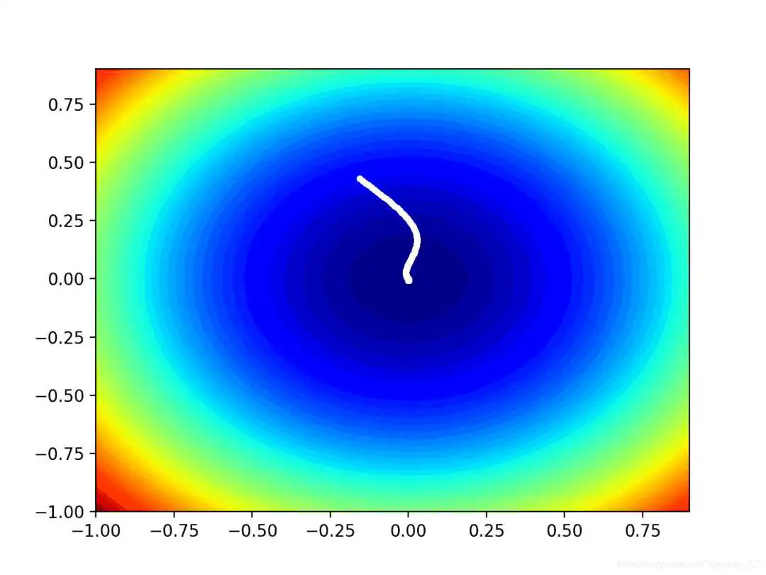
# create a filled contour plot with 50 levels and jet color scheme
pyplot.contourf(x, y, results, levels=50, cmap='jet')

最后，我们可以将在搜索过程中找到的每个解决方案绘制成一条由一条线连接的白点。

# plot the sample as black circles
solutions = asarray(solutions)
pyplot.plot(solutions[:, 0], solutions[:, 1], '.-', color='w')

综上所述，下面列出了对测试问题执行 Adam 优化并将结果绘制在轮廓图上的完整示例。

# example of plotting the adam search on a contour plot of the test function
from math import sqrt
from numpy import asarray
from numpy import arange
from numpy.random import rand
from numpy.random import seed
from numpy import meshgrid
from matplotlib import pyplot
from mpl_toolkits.mplot3d import Axes3D
 
# objective function
def objective(x, y):
 return x2.0 + y2.0
 
# derivative of objective function
def derivative(x, y):
 return asarray([x * 2.0, y * 2.0])
 
# gradient descent algorithm with adam
def adam(objective, derivative, bounds, n_iter, alpha, beta1, beta2, eps=1e-8):
 solutions = list()
 # generate an initial point
 x = bounds[:, 0] + rand(len(bounds)) * (bounds[:, 1] - bounds[:, 0])
 score = objective(x[0], x[1])
 # initialize first and second moments
 m = [0.0 for _ in range(bounds.shape[0])]
 v = [0.0 for _ in range(bounds.shape[0])]
 # run the gradient descent updates
 for t in range(n_iter):
  # calculate gradient g(t)
  g = derivative(x[0], x[1])
  # build a solution one variable at a time
  for i in range(bounds.shape[0]):
   # m(t) = beta1 * m(t-1) + (1 - beta1) * g(t)
   m[i] = beta1 * m[i] + (1.0 - beta1) * g[i]
   # v(t) = beta2 * v(t-1) + (1 - beta2) * g(t)^2
   v[i] = beta2 * v[i] + (1.0 - beta2) * g[i]2
   # mhat(t) = m(t) / (1 - beta1(t))
   mhat = m[i] / (1.0 - beta1(t+1))
   # vhat(t) = v(t) / (1 - beta2(t))
   vhat = v[i] / (1.0 - beta2(t+1))
   # x(t) = x(t-1) - alpha * mhat(t) / (sqrt(vhat(t)) + ep)
   x[i] = x[i] - alpha * mhat / (sqrt(vhat) + eps)
  # evaluate candidate point
  score = objective(x[0], x[1])
  # keep track of solutions
  solutions.append(x.copy())
  # report progress
  print('>%d f(%s) = %.5f' % (t, x, score))
 return solutions
 
# seed the pseudo random number generator
seed(1)
# define range for input
bounds = asarray([[-1.0, 1.0], [-1.0, 1.0]])
# define the total iterations
n_iter = 60
# steps size
alpha = 0.02
# factor for average gradient
beta1 = 0.8
# factor for average squared gradient
beta2 = 0.999
# perform the gradient descent search with adam
solutions = adam(objective, derivative, bounds, n_iter, alpha, beta1, beta2)
# sample input range uniformly at 0.1 increments
xaxis = arange(bounds[0,0], bounds[0,1], 0.1)
yaxis = arange(bounds[1,0], bounds[1,1], 0.1)
# create a mesh from the axis
x, y = meshgrid(xaxis, yaxis)
# compute targets
results = objective(x, y)
# create a filled contour plot with 50 levels and jet color scheme
pyplot.contourf(x, y, results, levels=50, cmap='jet')
# plot the sample as black circles
solutions = asarray(solutions)
pyplot.plot(solutions[:, 0], solutions[:, 1], '.-', color='w')
# show the plot
pyplot.show()

运行示例将像以前一样执行搜索，但是在这种情况下，将创建目标函数的轮廓图。

在这种情况下，我们可以看到在搜索过程中找到的每个解决方案都显示一个白点，从最优点开始，逐渐靠近图中心的最优点。

作者：沂水寒城，CSDN博客专家，个人研究方向：机器学习、深度学习、NLP、CV

Blog: http://yishuihancheng.blog.csdn.net

赞 赏 作 者

更多阅读

点击下方阅读原文加入社区会员

到此这篇梯度提升树算法流程（梯度提升算法的理解）的文章就介绍到这了,更多相关内容请继续浏览下面的相关推荐文章，希望大家都能在编程的领域有一番成就！

版权声明：

本文来自互联网用户投稿，该文观点仅代表作者本人，不代表本站立场。本站仅提供信息存储空间服务，不拥有所有权，不承担相关法律责任。
如若内容造成侵权、违法违规、事实不符，请将相关资料发送至xkadmin@xkablog.com进行投诉反馈，一经查实，立即处理！

转载请注明出处，原文链接：https://www.xkablog.com/jszy-jnts/18664.html